Statistical Analysis and Sampling Distribution

Welcome back!

Consider a population consisting of the following values, which represents the number of ice cream purchases during the academic year for each of the five housemates.
8, 14, 16, 10, 11

a. Compute the mean of this population.

INPUT

OUTPUT

So the mean would be 11.8

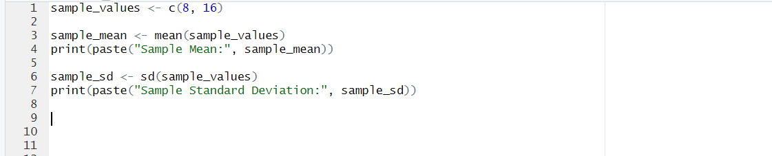
b. Select a random sample of size 2 out of the five members.

Let's randomly select two members from the population. For example, we could select 8 and 16

$$

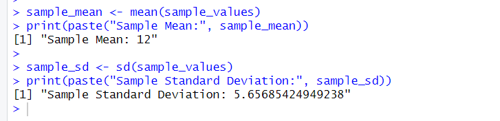
c. Compute the mean and standard deviation of your sample.

INPUT 

OUTPUT

d. Compare the Mean and Standard deviation of your sample to the entire population of this set (8,14, 16, 10, 11).

When comparing the sample to the entire population, we observe that the sample mean and population mean are quite similar. The population mean, calculated from the values $8, 14, 16, 10, 11$, is 11.8, while the mean of the selected sample ($8, 16$) is 12. This small difference shows that even with a sample size of 2, the sample mean can closely approximate the population mean. However, the standard deviation tells a different story. The population standard deviation is approximately 2.86, while the sample standard deviation is significantly higher at around 5.66. This larger sample standard deviation is due to the increased variability found in smaller samples. Smaller samples are more sensitive to extreme values, causing greater fluctuation in standard deviation, while larger populations tend to produce more stable estimates. Thus, while the means are close, the variability in the sample is much higher than in the population.

B.

Suppose that the sample size n = 100 and the population proportion p = 0.95.

1. Does the sample proportion p have approximately a normal distribution? Explain

For the sample proportion $\hat{p}$ to have an approximately normal distribution, the following conditions must be satisfied:

• $np$ must be greater than 5.
• $nq$ must be greater than 5.

Given:

• Sample size $n = 100$
• Population proportion $p = 0.95$
• $q = 1 - p = 0.05$

Now we calculate:

$$np = 100 \times 0.95 = 95$$ $$nq = 100 \times 0.05 = 5$$

Both $np = 95$ and $nq = 5$ are greater than or equal to 5. Thus, the sample proportion $\hat{p}$ can be considered to have an approximately normal distribution.

2. What is the smallest value of n for which the sampling distribution of p is approximately normal?   

1. To satisfy the normal approximation, both conditions $np > 5$ and $nq > 5$ must hold.

   $$np > 5 \implies n \times 0.95 > 5 \implies n > \frac{5}{0.95} \approx 5.26$$ $$nq > 5 \implies n \times 0.05 > 5 \implies n > \frac{5}{0.05} = 100$$

   Therefore, the smallest value of $n$ for which both conditions are satisfied is $n = 100$.

The sample mean  from a group of observations is an estimate of the population mean μ . Given a sample of size n, consider n independent random variables X1, X2, ..., Xn, each corresponding to one randomly selected observation. Each of these variables has the distribution of the population, with mean μ  and standard deviation σ .
A. Population mean= (8­­+14+16+10+11)/5 = 11.8

B. Sample of size n=  5
C. Mean of sample distribution:

Mean of Sample 1:

$$\text{Mean} = \frac{8 + 14 + 16 + 10 + 11}{5} = \frac{59}{5} = 11.8$$

Mean of Sample 2:

$$\text{Mean} = \frac{9 + 15 + 12 + 10 + 14}{5} = \frac{60}{5} = 12$$

Mean of Sample 3:

$$\text{Mean} = \frac{7 + 11 + 13 + 15 + 12}{5} = \frac{58}{5} = 11.6$$

And Standard Error Qm=Q/square root of n=4.4/square root of 5

D. I am looking for table with the following variables X, x=u, and 
(x-u)^2

Simulated coin tossing is probability better done using function called rbinom than using function called sample.  Explain.

Simulated coin tossing can be performed using both the rbinom and sample functions in R, but rbinom is often the better choice for efficiency and simplicity. The rbinom function directly generates random numbers from a binomial distribution, which is ideal for modeling the independent trials of coin tosses. By specifying the number of tosses and the probability of heads, you can easily simulate multiple tosses in a single function call. In contrast, the sample function requires you to define a vector of outcomes and can be less efficient, especially for larger sample sizes, as it generates each toss individually. While sample is versatile and can represent various outcomes, rbinom provides a more streamlined approach for straightforward scenarios like coin tossing, making it the preferred method for many statistical simulations.